Damped Oscillator
Differential Equation
The easiest assumption for a damped oscillator is friction that is proportional to its speed. In this case, the differential equation to solve can be written as
$$m\ddot{x} = - kx - r\dot{x}$$
Similar to the spring pendulum, the substitution $k/m = \omega_0^2$ can be made, where $\omega_0$ denotes the frequency of the undamped oscillator. Additionally, the value $r/m$ will be will replaced by $2\gamma$. Here, $\gamma$ represents the damping constant of the oscillator. Factor 2 has been inserted to make the following calculations easier. These replacements lead to the following important equation of motion for a damped oscillator
$$\boxed{\ddot{x} + 2\gamma \dot{x} + \omega_0^2x = 0}$$
In contrast to a spring pendulum, the simple ansatz of using a trigonometric function cannot be made anymore because of the additional derivation of $x$ with respect to time. However, the following ansatz will give the correct results:
$$x(t) = c e^{\lambda t}$$
where $c$ and $\lambda$ are just constants that have to be determined by inserting this function into the differential equation, leading to the following characteristic polynomial:
$$\lambda^2 +2\gamma\lambda + \omega_0^2 = 0$$
The solution to this second-degree polynomial can be found as
$$\lambda_{1,2} = -\gamma \pm \sqrt{\gamma^2-\omega_0^2}$$
This results in the following general solution
$$x(t) = e^{-\gamma t}\left(c_1e^{\sqrt{\gamma^2-\omega_0^2}}+c_2e^{-\sqrt{\gamma^2 - \omega_0^2}}\right)$$
There are now three possibilities for solutions which are described in the following.
Weak Damping
Weak damping can be considered if $\gamma < \omega_0$. In this case, the value $\lambda_{1,2}$ is given as
$$\lambda_{1,2} = -\gamma\pm \sqrt{-\omega_0^2} = -\gamma\pm \omega_0$$
which leads to the following solution
$$x(t) = Ae^{-\gamma t}\left(e^{i\omega_0 t}+e^{-i\omega_0 t}\right)$$
which can be written as
$$\boxed{x(t) = Ae^{-\gamma t}\cos\omega_0 t}$$
The additional phase $\varphi$ in the cosine function has been neglected. This very important result indicates that the amplitude of a damped oscillator decreases exponentially.
Strong Damping
The next case is the so-called strong damping which takes place if $\gamma > \omega_0$. The constants $\lambda_{1,2}$ can then be written as
$$\lambda_{1,2} = -\gamma \pm \sqrt{\gamma^2 - \omega_0^2} = -\gamma \pm \alpha$$
where $\alpha$ replaces the $\sqrt{\gamma^2 - \omega_0^2}$. Since the exponents are now real numbers, the function $x(t)$ can now be written as
$$x(t) = e^{-\gamma t}\left(c_1e^{\alpha t} + c_2e^{-\alpha t}\right)$$
Using the boundary condition $x(t) = 0$ and $\dot{x}(t) = v_0$ leads to
$$x(t) = \frac{v_0}{2\alpha}e^{-\gamma t}\left(e^{\alpha t} + e^{-\alpha t}\right)$$
Using the definition of the sine hyperbolic gives
$$\boxed{x(t) = Ae^{-\gamma t}\sinh\alpha t}$$
where $A$ replaces the factor $v_0/\alpha$.
Critical Damping
Finally, we take a look at the so-called critical damping, where the condition $\gamma = \omega_0$ is fulfilled. Now, both constants $\lambda_{1,2}$ are qual to $-\gamma$. This results in the following special solution
$$\boxed{x(t) = A(1+\gamma t)e^{-\gamma t}}$$
As one can see, the critical damping is the one with the fastest decline in amplitude and therefore often used for dampers in cars to make sure that they come to rest very quick after shaking starts
This page contains 657 words and 4110 characters.
Last modified: 2022-10-01 17:10:27 by mustafa
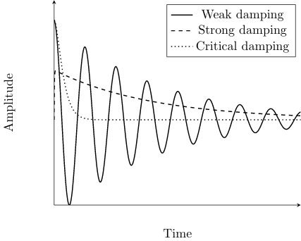 All three damping possibilities.

